Advection solvers
The linear advection equation:
provides a good basis for understanding the methods used for compressible hydrodynamics. Chapter 4 of the notes summarizes the numerical methods for advection that we implement in pyro.
pyro has several solvers for linear advection:
advectionimplements the directionally unsplit corner transport upwind algorithm with piecewise linear reconstructionadvection_fv4uses a fourth-order accurate finite-volume method with RK4 time integrationadvection_rkuses a method of lines time-integration approach with piecewise linear spatial reconstruction for linear advectionadvection_wenouses a WENO reconstruction and method of lines time-integration
The main parameters that affect this solver are:
[driver] |
|
|---|---|
cfl |
the advective CFL number (what fraction of a zone can we cross in a single timestep) |
[advection] |
|
|---|---|
u |
the advective velocity in the x direction |
v |
the advective velocity in the y direction |
limiter |
what type of limiting to use in reconstructing the slopes. 0 means use an unlimited second-order centered difference. 1 is the MC limiter, and 2 is the 4th-order MC limiter |
temporal_method |
the MOL integration method to use (RK2, TVD2, TVD3, RK4) (advection_rk only) |
The main use for the advection solver is to understand how Godunov techniques work for hyperbolic problems. These same ideas will be used in the compressible and incompressible solvers. This video shows graphically how the basic advection algorithm works, consisting of reconstruction, evolution, and averaging steps:
Examples
smooth
The smooth problem initializes a Gaussian profile and advects it with \(u = v = 1\) through periodic boundaries for a period. The result is that the final state should be identical to the initial state—any disagreement is our numerical error. This is run as:
./pyro.py advection smooth inputs.smooth
By varying the resolution and comparing to the analytic solution, we
can measure the convergence rate of the method. The smooth_error.py
script in analysis/ will compare an output file to the analytic
solution for this problem.
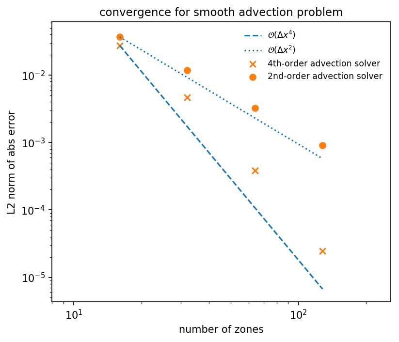
The points above are the L2-norm of the absolute error for the smooth
advection problem after 1 period with CFL=0.8, for both the
advection and advection_fv4 solvers. The dashed and dotted
lines show ideal scaling. We see that we achieve nearly 2nd order
convergence for the advection solver and 4th order convergence
with the advection_fv4 solver. Departures from perfect scaling
are likely due to the use of limiters.
tophat
The tophat problem initializes a circle in the center of the domain with value 1, and 0 outside. This has very steep jumps, and the limiters will kick in strongly here.
Exercises
The best way to learn these methods is to play with them yourself. The exercises below are suggestions for explorations and features to add to the advection solver.
Explorations
- Test the convergence of the solver for a variety of initial conditions (tophat hat will differ from the smooth case because of limiting). Test with limiting on and off, and also test with the slopes set to 0 (this will reduce it down to a piecewise constant reconstruction method).
- Run without any limiting and look for oscillations and under and overshoots (does the advected quantity go negative in the tophat problem?)
Extensions
Implement a dimensionally split version of the advection algorithm. How does the solution compare between the unsplit and split versions? Look at the amount of overshoot and undershoot, for example.
Research the inviscid Burger’s equation—this looks like the advection equation, but now the quantity being advected is the velocity itself, so this is a non-linear equation. It is very straightforward to modify this solver to solve Burger’s equation (the main things that need to change are the Riemann solver and the fluxes, and the computation of the timestep).
The neat thing about Burger’s equation is that it admits shocks and rarefactions, so some very interesting flow problems can be setup.